ONNX at Auction Speed: Packaging ML Pipelines for Real-Time Bidding

At Digital Turbine, we operate one of the world’s largest independent mobile advertising platforms. Through our App Growth Platform (AGP), we connect thousands of publishers and app developers with advertisers via programmatic, real-time bidding (RTB) auctions — processing hundreds of billions of ad requests every day across devices, carriers, and OEMs worldwide.

The engine behind this is a decision that has to happen in under 100 milliseconds: given an auction opportunity, what should we bid? That window encompasses network round-trips, fraud detection, audience matching, and — the subject of this post — a machine learning inference call that predicts the value of the impression.

The scale of modern RTB systems is staggering. Industry measurements put peak programmatic auction traffic above 12 million bid requests per second. Every millisecond of latency at that scale directly affects win rates and revenue. At this throughput, a model that adds even 5ms of overhead can cost millions of missed auction opportunities per day.

To build the models that power these decisions, our data science teams process weeks of auction logs at terabyte scale — billions of auction events per training window. At this volume, distributed training is not optional; it is the only viable path. We train both classical ML models and deep learning models for different parts of the decision pipeline.

The challenge, however, is not training — it is serving.

The Latency Wall

Python is an extraordinary language for machine learning. Its ecosystem — NumPy, pandas, scikit-learn, XGBoost, PyTorch — makes experimentation fast and expressive. But Python is not fast at serving time. A production backend written in Java, Scala, C++, Rust, or Go cannot simply import standard ML libraries like scikit-learn or XGBoost, or call into a distributed training pipeline. Even if it could, loading such infrastructure in the hot path of an auction is not an option.

There is another, subtler problem: the gap between training and serving code. A production ML pipeline is rarely just a model. It includes:

• Preprocessing: categorical feature encoding, string indexing, normalization, scaling
• Feature engineering: derived features, time-based features, ratio features
• Postprocessing: clamping outputs to valid ranges, inverting target transformations to return predictions in the original scale

Traditionally, data scientists implement these steps in Python for training, then hand the model weights to a backend team who re-implements the same logic in another language. This creates a persistent risk: any discrepancy between the Python preprocessing and the production implementation causes training-serving skew — predictions that differ between offline evaluation and live traffic, silently, without an obvious error.

ONNX to the Rescue

ONNX (Open Neural Network Exchange) is an open standard for representing ML models and computational graphs. Originally designed to allow models to move between deep learning frameworks (PyTorch ↔ TensorFlow), it has matured into something much more powerful: a portable, runtime-agnostic computation graph that can encode not just model weights but arbitrary tensor operations — including all the preprocessing and postprocessing steps that surround the model.

The key insight is this: the entire pipeline — from raw request inputs to final bid-price prediction — can be compiled into a single .onnx file. The data science team owns and maintains this file. The backend team calls one function: session.run(raw_inputs). No re-implementation. No drift.

In this post, we walk through exactly how we do this, using a toy example built on data from our public Kaggle auction bid-price prediction competition. We will cover:

1. Feature engineering in Spark and why certain transforms are necessary.
2. Training a distributed XGBoost model with SparkXGBRegressor.
3. Exporting a metadata contract that drives the ONNX graph.
4. Constructing a four-stage ONNX graph: preprocessing → XGBoost → merge → postprocessing.
5. Debugging tools: describe_graph, Netron, and ONNX Runtime traces.
6. Serving with ONNX Runtime in single-row and batch modes.

The full code is available in our GitLab repository.

Why ONNX and Not Something Else?

ONNX is not the only option for bridging the Python-to-production gap. So why not:

• TorchScript / TorchServe? Excellent for PyTorch-native deep learning models, but they require LibTorch as a C++ dependency — significantly heavier than ONNX Runtime, and less standard in polyglot backend environments.
• Custom C++ implementations? Direct model C++ APIs exist and are fast, but backend engineers must manage the model format, versioning, and all preprocessing logic — recreating the exact ownership problem we are trying to solve.
• Model-specific export formats (e.g., XGBoost JSON)? Lightweight, but model weights only. Preprocessing still needs to be re-implemented on the backend side.
• NVIDIA Triton Inference Server? A more complete inference package with quality-of-life features like automatic micro-batching and model management, and native support for both ONNX and dedicated GBT backends (FIL — Forest Inference Library). We benchmarked ONNX Runtime directly against Triton and found the performance overhead and operational complexity weren’t justified for our use case: we only needed specific capabilities, so we built exactly that around it — lighter, purpose-fit, and nothing we don’t use.

ONNX’s advantage is its generality: it is not tied to any single framework, runs in a lightweight runtime available in every major language, and can represent arbitrary preprocessing logic alongside the model. That combination — one file, one runtime call, full pipeline — is what makes it the right architectural choice here.

The Ownership Problem

Before diving into code, it is worth being precise about the problem we are solving.

A typical ML model deployment in an ad tech company looks like this:

Re-implementing pre- and postprocessing is where bugs live. These steps are also where ownership is ambiguous: when a prediction looks wrong in production, is it the model, the preprocessing, or the postprocessing? Which team’s bug is it?

The ONNX approach consolidates ownership:

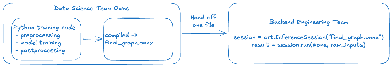
The backend team receives a versioned, validated artifact. There is nothing to re-implement. The data science team can update transformations, retrain the model, and ship a new .onnx file — all without changing a line of backend code.

A further benefit: because the preprocessing is encoded as ONNX operators rather than re-implemented in a separate language, it directly represents the same computation — the same graph structure, the same initializer values, the same operator semantics. This eliminates the primary source of training-serving skew: divergent re-implementations. Minor numerical differences from floating-point precision (ONNX uses 32-bit floats) or platform variations remain possible, but are far easier to detect and test when a single team owns the full pipeline.

Key takeaway: ONNX moves the preprocessing/postprocessing ownership boundary from "split between two teams" to "fully owned by data science, consumed as a black box by backend."

The Dataset: Digital Turbine Auction Bid Price Prediction

For this walkthrough we use the dataset from our public Kaggle competition. This is real (anonymized) auction data from our exchange, and it gives us a natural use case: predicting the winning bid price (winBid) for an auction given the features known at bid time.

Key columns:

• ‍unitDisplayType, string. Ad placement type: banner, interstitial, or rewarded.
• ‍countryCode, string. ISO country code of the user (e.g., US, DE, JP).
• ‍eventTimestamp, long. Epoch timestamp in milliseconds.
• ‍sentPrice, double. The bid floor price sent by the exchange.
• ‍winBid, double. Target: the actual auction clearing price.

This is a regression problem: predict a continuous bid price value. The task sounds simple, but the raw distributions are far from well-behaved — a reality we address with feature engineering.

Note that the model we build here is a toy example designed to illustrate the ONNX pipeline pattern. It is not intended to represent our production bid-price model, which incorporates many additional signals and a more sophisticated architecture.

From "Why" to "How": Having covered the problem — training-serving skew, ownership fragmentation, and the latency wall — the rest of this post is a concrete technical walkthrough. We have deliberately kept the example simple to make the ONNX workflow as legible as possible. Our production pipelines are significantly more complex, but the same patterns apply at scale. Along the way, we highlight Key Takeaways and common pitfalls encountered in large-scale data environments.

Feature Engineering in Spark

All feature engineering runs inside a Spark Pipeline on a Databricks cluster. This is important for two reasons: (1) the data volume requires distributed processing, and (2) the fitted pipeline stages (e.g., StringIndexerModel, OneHotEncoderModel) carry the vocabulary and encoding metadata that we will later bake directly into the ONNX graph.

Time Features: Cyclic Hour Encoding

To illustrate how time-based features integrate into the pipeline, consider a common ad-tech challenge: representing time-of-day in a way that preserves its cyclic nature. Many techniques exist (embedding lookup, linear binning, learned positional encodings), but we demonstrate a sine/cosine approach that is simple, compact, and native to ONNX operators. We extract the hour of day from eventTimestamp (milliseconds epoch) and convert it to two cyclic features:

hour_sin = sin(2π × hour / 24)
hour_cos = cos(2π × hour / 24)

Why cyclic? A naive integer hour (0–23) encodes hour 23 and hour 0 as far apart when they are actually adjacent. Sine and cosine together form a continuous cyclic representation: the angular distance between any two hours is proportional to their true temporal distance on a 24-hour clock. Using periodic functions as feature representations for time is well-motivated in the ML literature.

# From FeatureEngineering.add_time_features() in utils.py
df = (
    df
    .withColumn(sin_col, F.sin(F.lit(2.0 * math.pi) * F.col(hour_col) / F.lit(24.0)))
    .withColumn(cos_col, F.cos(F.lit(2.0 * math.pi) * F.col(hour_col) / F.lit(24.0)))
)

These two features encode both amplitude and phase of the daily cycle, so XGBoost can learn patterns like "high bids in the late evening" without needing to hard-code time boundaries.

Power Transform: Taming Skewed Bid Distributions

To illustrate how feature engineering handles skewed distributions — a challenge endemic to ad-tech data — consider the winBid and sentPrice columns. While many normalisation techniques exist (log transform, quantile transform, rank-based scaling), we demonstrate a power transform approach that fits naturally into our ONNX postprocessing story: because the transform is invertible, we can encode both the forward and inverse steps into the same graph. Auction bid prices are heavily right-skewed. A small number of premium placements command prices an order of magnitude higher than the median. This kind of distribution is a known challenge for tree-based models: the model can spend most of its splits trying to resolve the long tail rather than learning general patterns in the bulk of the distribution.

The raw winBid distributions by placement type (top row) show exactly this shape: nearly all values cluster near zero with a long tail to the right. The power-transformed versions (bottom row) are far more symmetric and easier for a model to learn from.

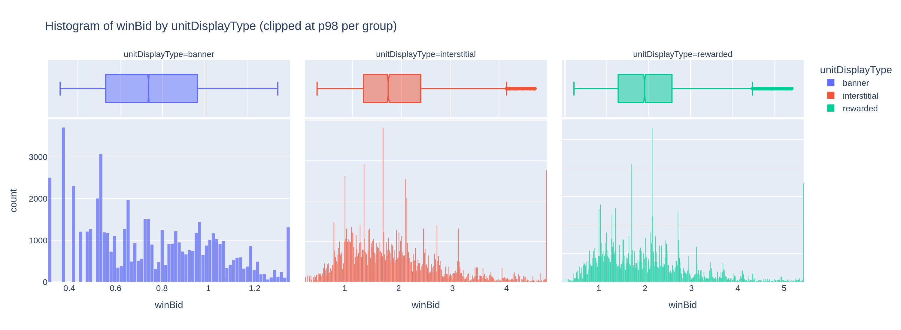
We apply a per-placement-type power transform of the form x^(1/n) where n is tuned per placement category. This is a restricted form of the Box-Cox power transform family, constrained to positive-only inputs (which bid prices always are). Recent work on applying power transforms in machine learning contexts confirms that such transformations can significantly improve model accuracy by normalizing the input distribution.

The exponents are defined in config.py and can be fine-tuned as part of a hyperparameter tuning process:

POWER_N: Dict[str, float] = {
    "banner":       4.0,
    "interstitial": 3.0,
    "rewarded":     3.0,
}
POWER_N_DEFAULT: float = 3.0

The transform is applied both to the input feature sentPrice and to the target winBid. Critically, since the model learns in transformed space, any prediction it outputs is also in transformed space — we must invert the transform at serving time to get a prediction in the original bid-price scale. This is the postprocessing step we will encode into the ONNX graph.

# From FeatureEngineering.power_transform() in utils.py
for c in cols:
    df = df.withColumn(f"{c}_orig", F.col(c))  # keep original for comparison
    exponent = F.lit(1.0 / default_n)
    for group, n in power_n_by_group.items():
        exponent = F.when(
            F.col(group_col) == F.lit(group),
            F.lit(1.0 / float(n))
        ).otherwise(exponent)
    df = df.withColumn(
        c,
        F.pow(F.greatest(F.col(c), F.lit(0.0)), exponent)
    )

‍Categorical Encoding

Placement type (unitDisplayType) goes through StringIndexer → OneHotEncoder (with dropLast=True to avoid dummy variable collinearity). Because the Spark encoder uses handleInvalid="keep", it reserves an extra bucket for unseen labels at serving time — a useful safety net in production where new placement types may appear.

Country code (countryCode) is encoded with StringIndexer only — producing a float index (0, 1, 2, …) rather than a one-hot vector. Given that there can be 200+ distinct countries in our data, one-hot encoding would add excessive dimensionality for what is essentially a ranking signal. The index encoding still lets XGBoost learn country-specific effects via its tree splits.

Feature Vector: A Deterministic, Ordered Contract

The assembled feature vector follows a fixed order defined as a single source of truth in config.py:

FEATURE_INPUT_COLS_ORDER: List[str] = [
    "placement_ohe",   # one-hot vector, variable width depending on # placement types
    "country_idx",     # scalar float
    "hour_sin",        # scalar float
    "hour_cos",        # scalar float
    "sentPrice",       # scalar float (power-transformed)
]

This order is critical. The Spark VectorAssembler produces features in this order, the XGBoost model is trained on features in this order, and the ONNX preprocessing graph must produce a features tensor in exactly this order. Any mismatch would silently feed the wrong values to the wrong tree splits — a bug that would be very hard to detect.

Key takeaway: Define feature order once, in a config, and reference it everywhere: training, metadata export, and ONNX graph construction.

Training a Distributed XGBoost Model

With features engineered, we train a gradient-boosted tree model — specifically SparkXGBRegressor from the XGBoost PySpark API. We chose this model family because it represents the "classical ML" archetype well: non-neural, tree-based, and widely used in ad-tech prediction tasks. The ONNX export pattern we demonstrate here applies equally to other classical ML frameworks. Our production pipelines mirror these same patterns at a larger scale.

The full pipeline is:

Pipeline(stages=[
    StringIndexer(inputCol="unitDisplayType", outputCol="placement_idx", handleInvalid="keep"),
    OneHotEncoder(inputCols=["placement_idx"], outputCols=["placement_ohe"], handleInvalid="keep"),
    StringIndexer(inputCol="countryCode", outputCol="country_idx", handleInvalid="keep"),
    VectorAssembler(inputCols=FEATURE_INPUT_COLS_ORDER, outputCol="features"),
    SparkXGBRegressor(
        features_col="features",
        label_col="winBid",
        validation_indicator_col="is_validation",
        objective="reg:squarederror",
        max_depth=6,
        eta=0.08,
        num_round=200,
        subsample=0.8,
        colsample_bytree=0.8,
        callbacks=[CollectEval(period=25)],
    )
])

The validation_indicator_col mechanism deserves mention. Rather than a random train/val split, we use a time-based split: the most recent 20% of events (by eventTimestamp) become the validation set. This mimics the real-world scenario where a model trained on historical data is evaluated on future auctions. Train/test splitting is a domain unto itself — random splits, time-based splits, group-based splits, and stratified variants each reflect different assumptions about the problem. We use a time-based split here because it best reflects our production environment and the real-world temporal dynamics discussed earlier. The CollectEval callback captures RMSE at every boosting round so we can visualize the training curve.

Exporting the Preprocessing Metadata

Before building the ONNX graph, we export a metadata JSON file that captures all the information needed to reconstruct the preprocessing steps exactly. This file is the contract between the Python training code and the ONNX builder.

From PreprocMetadataWriter.build_metadata() in utils.py:

{
  "opset": 17,
  "feature_order": ["placement_ohe", "country_idx", "hour_sin", "hour_cos", "sentPrice"],
  "power_transform": {
    "enabled": true,
    "group_col": "unitDisplayType",
    "power_n_by_group": {"banner": 4.0, "interstitial": 3.0, "rewarded": 3.0},
    "default_n": 3.0,
    "cols": ["sentPrice", "winBid"]
  },
  "target_normalization": {"enabled": true},
  "notes": {
    "placement_ohe_expands": true,
    "country_idx_is_float": true,
    "hour_features": ["hour_sin", "hour_cos"]
  }
}

Every coefficient and label mapping the ONNX builder uses comes from this file (and from the fitted pipeline stages). Nothing is hardcoded in the ONNX builder itself. If you retrain the model on new data with different country vocabulary or different power-transform exponents, you regenerate the metadata and rebuild the graph — the ONNX construction code stays unchanged.

Key takeaway: The metadata JSON is the single source of truth for all preprocessing parameters. It bridges training and graph construction and should be versioned alongside the model artifact.

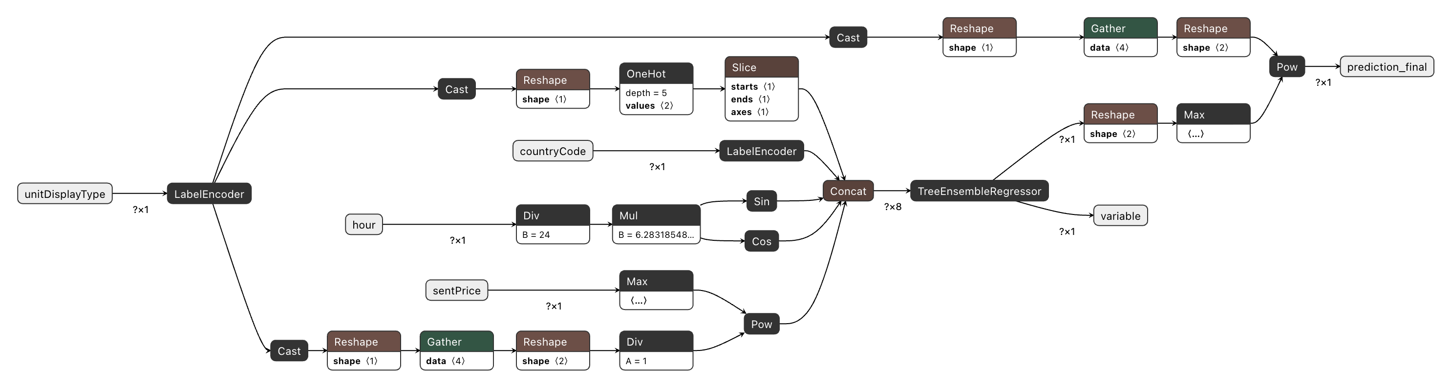
Building the ONNX Graph: Four Stages

Now for the heart of the post. We construct the ONNX graph in four stages, each building on the previous.

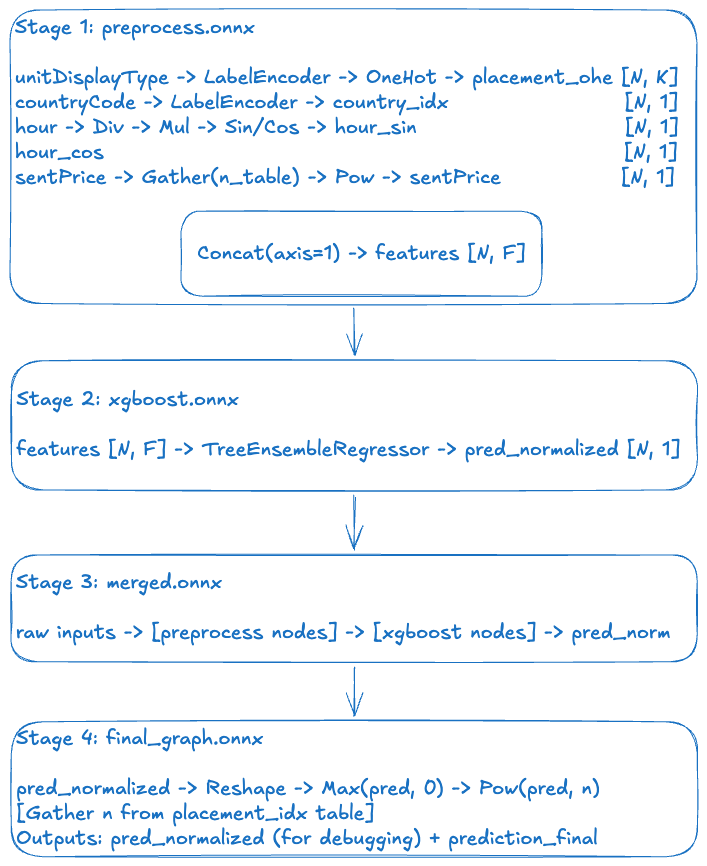
Stage 1: Preprocessing Graph

The preprocessing graph is built by hand using the ONNX helper API, directly translating each Spark pipeline stage into ONNX operators. The OnnxBlogpostGraphBuilder class in utils.py handles this.

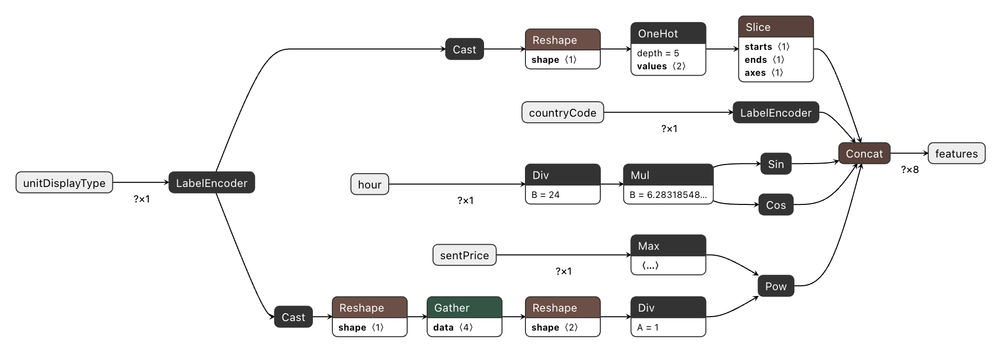
Label encoding (placement type):

The fitted StringIndexerModel carries the vocabulary as an ordered list (labels). We create an ai.onnx.ml.LabelEncoder node that maps each string to a float index, with known labels assigned indices 0, 1, … and unseen strings assigned a default_float index (equal to the vocabulary size — the "unknown" bucket):

helper.make_node(
    "LabelEncoder",
    inputs=["unitDisplayType"],
    outputs=["placement_idx"],
    domain="ai.onnx.ml",
    keys_strings=["banner", "interstitial", "rewarded"],
    values_floats=[0.0, 1.0, 2.0],
    default_float=3.0,   # unseen label → index 3
)

‍One-hot encoding:

We Cast the float index to int64, Reshape to a 1-D vector, then apply the ONNX OneHot operator. If dropLast=True (our default, to avoid collinearity), we append a Slice node that removes the last column:

# Cast → Reshape → OneHot → Slice (dropLast)
helper.make_node("Cast",    ["placement_idx"],        ["placement_idx__i64"],   to=TensorProto.INT64)
helper.make_node("Reshape", ["placement_idx__i64",    "shape_minus1"],          ["placement_idx__1d"])
helper.make_node("OneHot",  ["placement_idx__1d",     "ohe_depth", "ohe_vals"], ["placement_ohe__raw"], axis=-1)
helper.make_node("Slice",   ["placement_ohe__raw",    "starts", "ends", "axes"],["placement_ohe"])

‍Country code: Same LabelEncoder pattern, without the subsequent OneHot step.

Cyclic hour features:

helper.make_node("Div", ["hour",      "const_24"],   ["hour_norm"])
helper.make_node("Mul", ["hour_norm", "const_2pi"],  ["hour_angle"])
helper.make_node("Sin", ["hour_angle"],              ["hour_sin"])
helper.make_node("Cos", ["hour_angle"],              ["hour_cos"])

Constants (24.0, 2π) are stored as ONNX initializers — tensor constants baked into the graph.

Placement-dependent power transform for sentPrice:

This is the most interesting piece. Rather than a fixed exponent, we need n to vary by placement type. The solution is a lookup table (initializer) indexed by the placement index:

# n_table = [4.0, 3.0, 3.0, 3.0]  (banner, interstitial, rewarded, unknown)
helper.make_node("Cast",    ["placement_idx"],               ["placement_idx__i64__pow"],  to=TensorProto.INT64)
helper.make_node("Reshape", ["placement_idx__i64__pow",      "shape_minus1"],              ["placement_idx__1d__pow"])
helper.make_node("Gather",  ["placement_power_n_table",      "placement_idx__1d__pow"],    ["placement_power_n__1d"],  axis=0)
helper.make_node("Reshape", ["placement_power_n__1d",        "shape_n1"],                  ["placement_power_n__2d"])
# exponent = 1/n
helper.make_node("Div",     ["const_one", "placement_power_n__2d"], ["placement_power_inv_n"])
# sentPrice^(1/n)
helper.make_node("Max",     ["sentPrice", "const_zero"],     ["sentPrice__nonneg"])
helper.make_node("Pow",     ["sentPrice__nonneg",            "placement_power_inv_n"],      ["sentPrice__pow"])

Feature vector concatenation:

Finally, all feature tensors are concatenated in the canonical order:

helper.make_node(
    "Concat",
    inputs=["placement_ohe", "country_idx", "hour_sin", "hour_cos", "sentPrice__pow"],
    outputs=["features"],
    axis=1,
)

The feature order must exactly match the FEATURE_INPUT_COLS_ORDER used during Spark training. Any deviation is a silent correctness bug. Because both the Spark assembler and the ONNX builder read from the same config constant, this is enforced automatically.

Stage 2: XGBoost ONNX Graph

The trained XGBoost booster is converted via ONNXMLTools:

from onnxmltools import convert_xgboost
from onnxmltools.convert.common.data_types import FloatTensorType

xgb_onnx = convert_xgboost(
    booster,
    initial_types=[("features", FloatTensorType([None, feature_dim]))],
)

This produces a graph containing a TreeEnsembleRegressor node (from the ai.onnx.ml domain) that encodes all the tree structure and leaf values. The input is our features tensor of shape [N, F]; the output is the predicted value in normalized (power-transformed) space.

Stage 3: Merging the Graphs

onnx.compose.merge_models stitches the two graphs together by wiring the preprocessing output (features) to the XGBoost input:

xgb_input_name = xgb_onnx.graph.input[0].name   # e.g., "features" or "input"
merged = merge_models(
    preproc_onnx,
    xgb_onnx,
    io_map=[("features", xgb_input_name)],
)

After merging, features is no longer a graph-level output — it becomes an internal tensor, invisible from outside. The merged graph exposes only the original raw inputs and the XGBoost prediction output.

Stage 4: Inverse Power Transform (Postprocessing)

The model was trained on winBid^(1/n), so its output is in transformed space. To get a bid price in the original scale we append the inverse: max(0, pred)^n, where n is again looked up per placement type using the same initializer table approach:

# Tensors with the __inv suffix belong to the inverse-transform block
g.node.extend([
    helper.make_node("Cast",    ["placement_idx"],              ["placement_idx__i64__inv"],  to=TensorProto.INT64),
    helper.make_node("Reshape", ["placement_idx__i64__inv",     "shape_minus1__inv"],         ["placement_idx__1d__inv"]),
    helper.make_node("Gather",  ["placement_power_n_table__inv","placement_idx__1d__inv"],    ["placement_power_n__1d__inv"], axis=0),
    helper.make_node("Reshape", ["placement_power_n__1d__inv",  "shape_n1__inv"],             ["placement_power_n__2d__inv"]),
])
g.node.append(helper.make_node("Reshape", [pred_name, "shape_n1__inv"], [pred_2d]))
g.node.append(helper.make_node("Max",     [pred_2d,   "const_zero__inv"],                    [pred_nonneg]))
g.node.append(helper.make_node("Pow",     [pred_nonneg, "placement_power_n__2d__inv"],       ["prediction_final"]))

The final graph has two outputs: the raw normalized prediction (useful for debugging against the Spark evaluator’s RMSE), and prediction_final — the bid price in the original dollar-scale that the backend system actually uses.

Opset Versioning: A Critical Gotcha

When you merge two ONNX graphs, they must agree on the opset version for each domain. A preprocessing graph built with onnx==1.15 defaults and an XGBoost graph produced by ONNXMLTools may carry different opset_import entries — ONNX will reject the merge with an explicit error rather than silently producing a broken graph.

The root cause is tooling lag: converter libraries like ONNXMLTools do not always keep pace with ONNX releases. This creates two practical problems. First, mismatched defaults between tools cause merge errors that must be resolved by normalising opsets manually. Second, if a tool pins an older opset, you cannot use recently-added operators without bumping versions yourself — for example, StringConcat (added in main opset 20) or TreeEnsemble (added in ai.onnx.ml opset 5 in 2024, with significant improvements over the legacy TreeEnsembleRegressor and TreeEnsembleClassifier nodes, though not yet supported by ONNXMLTools).

We solve this with a single helper applied to every sub-graph before any merge:

# apply_onnx_model_config() in utils.py
model = set_domain_opset(model, "",            cfg.ONNX_OPSET)        # 17
model = set_domain_opset(model, "ai.onnx.ml",  cfg.ML_OPSET_VERSION)  # 3
model.ir_version = int(cfg.IR_VERSION)                                # 10

All three values — ONNX_OPSET, ML_OPSET_VERSION, and IR_VERSION — are defined in config.py and applied to every graph: the hand-built preprocessing graph, the ONNXMLTools-converted XGBoost graph, and the merged/final graph. This guarantees that merge_models always operates on compatible graphs. A secondary benefit: explicit pinning prevents accidental version bumps when Python packages are upgraded — important because the inference server runtime is managed independently and may not yet support newer opsets or IR versions. ONNX Runtime maintains backward compatibility with older opsets and IR versions, so pinning conservatively is a safe default.

Key takeaway: Always normalise the opset and IR version across all sub-graphs before merging. Define these as config constants and apply them centrally rather than relying on converter defaults.

Debugging the ONNX Graph (or: How We Taught an AI Agent to Read Our Nodes)

An ONNX graph can contain dozens or hundreds of nodes. Without good tooling, debugging one is painful. We use three tools.

describe_graph: Human-Readable Graph Summary

We wrote a describe_graph utility that prints a compact summary of any ONNX model, making it easy to quickly understand the graph structure and share it for debugging — including with AI assistants:

describe_graph(final_graph, "final", max_nodes=120, verbosity=1)

Output:

===== final =====
graph_name=blogpost_preprocess
nodes=47  initializers=18

inputs:
  - unitDisplayType
  - countryCode
  - hour
  - sentPrice

outputs:
  - variable       ← XGBoost raw output (normalized space)
  - prediction_final  ← bid price in original scale

At verbosity=2 it lists every node with its op type, letting you trace the full computation graph as text. This is particularly useful when pasting the output into a chat with an AI assistant to diagnose a construction issue or an unexpected output shape.

We also provide print_preprocess_data_flow() which prints a detailed breakdown of each feature segment:

PREPROCESS DATA FLOW (for debugging)
--- 5) FEATURE ORDER AND DIMENSIONS ---
  placement_ohe: dim = 3  (cumulative start index: 0)
  country_idx:   dim = 1  (cumulative start index: 3)
  hour_sin:      dim = 1  (cumulative start index: 4)
  hour_cos:      dim = 1  (cumulative start index: 5)
  sentPrice:     dim = 1  (cumulative start index: 6)
  Total feature dim F = 7

This tells you exactly which index in the features vector corresponds to which input — critical for verifying that the tree model received the right data.

Netron: Visual Graph Explorer

Netron is a browser-based ONNX graph visualizer. Upload any .onnx file and get an interactive, clickable node graph.

It is invaluable for:

• Tracing the preprocessing path: open preprocess.onnx, follow unitDisplayType through LabelEncoder → Cast → Reshape → OneHot → Slice → Concat
• Inspecting initializer values: click the placement_power_n_table initializer to verify the n-values match your config
• Finding the inverse transform block: in final_graph.onnx, search for the Pow node at the bottom of the graph and confirm it reads from the same placement index as the forward transform

A recommended workflow is to export all four pipeline stages (Stage 1–4) as separate .onnx files, which we do with onnx.save(), and inspect them one by one in Netron to validate each layer of the pipeline before running inference.

run_and_dump: Single-Row Trace

The run_and_dump helper runs an ONNX Runtime session on a test input and prints dtype, shape, and a value preview for each output tensor:

inputs_single = {
    "unitDisplayType": np.array([["banner"]]).astype(object),
    "countryCode":     np.array([["US"]]).astype(object),
    "hour":            np.array([[12.0]], dtype=np.float32),
    "sentPrice":       np.array([[0.7]],  dtype=np.float32),
}

preproc_results = run_and_dump(preproc_session, inputs_single, ["features"], "preprocess")

Output:

===== RUN: preprocess =====
features: dtype=float32, shape=(1, 7), preview=[1. 0. 0. 47. 0. 1. 0.5916]

Combined with print_preprocess_feature_vector, you get a named breakdown of exactly what values the model receives for each feature slot — making it easy to check that "banner at hour 12 with sentPrice=0.7" produces the expected one-hot encoding and transformed price.

Key takeaway: describe_graph + Netron + run_and_dump give you three complementary views of the graph: structural, visual, and numerical. Use all three when debugging a new pipeline.

Inference with ONNX Runtime

Once the final_graph.onnx is exported, Python is no longer in the serving path. The graph runs in ONNX Runtime (ORT) — a lightweight, cross-platform inference engine optimized for low-latency prediction, with backends in Python, Java, C#, C++, and JavaScript.

Creating a Session

import onnxruntime as ort

session = ort.InferenceSession(
    "final_graph.onnx",
    providers=["CPUExecutionProvider"]
)

Note that the snippets in this section use Python for legibility — the same .onnx file is consumed via an identical session.run() call from any supported runtime. In production, latency-sensitive inference typically runs outside of Python; our backend uses Rust via the ort crate, which wraps the same C++ ONNX Runtime under the hood. As an added benefit, ONNX Runtime applies graph-level optimizations at session load time that can make even Python inference faster than calling the original model’s native predict() directly.

The session is stateless and thread-safe. In a production service, create it once at startup and call session.run() for each incoming auction request. However, in some language bindings, e.g., Rust’s ort crate, run() requires exclusive mutable access — the standard pattern there is a session pool with one instance per worker thread. ORT also supports hardware-accelerated providers — swap "CPUExecutionProvider" for "CUDAExecutionProvider", "TensorrtExecutionProvider", or "CoreMLExecutionProvider" depending on your inference hardware, with no changes to the graph or calling code.

Single-Row Inference (Online Bidding)

In a real-time auction, one request arrives at a time. The input tensors have shape [1, 1] for both string and float inputs:

inputs_single = {
    "unitDisplayType": np.array([["banner"]]).astype(object),
    "countryCode":     np.array([["US"]]).astype(object),
    "hour":            np.array([[12.0]], dtype=np.float32),
    "sentPrice":       np.array([[0.7]],  dtype=np.float32),
}

outputs = session.run(None, inputs_single)
pred_normalized    = outputs[0]  # shape (1,)   — raw XGBoost score in transformed space, for diagnostics
prediction_final   = outputs[1]  # shape (1, 1) — bid price in original scale (note: 2D, unlike the 1D xgb output)
print(f"Predicted bid: {prediction_final[0][0]:.4f}")

Batch Inference (Offline Scoring / Shadow Mode)

The exact same session and exact same graph handle batches of arbitrary size N. No code changes, no graph modifications:

inputs_batch = {
    "unitDisplayType": np.array([["interstitial"], ["banner"], ["rewarded"]]).astype(object),
    "countryCode":     np.array([["US"], ["CA"], ["DE"]]).astype(object),
    "hour":            np.array([[12.0], [4.0], [20.0]], dtype=np.float32),
    "sentPrice":       np.array([[0.7],  [0.3], [1.2]],  dtype=np.float32),
}

batch_outputs = session.run(None, inputs_batch)
predictions = batch_outputs[1]  # shape (3, 1)

‍

This batching is not just a convenience — ONNX Runtime executes all preprocessing nodes and the tree-ensemble regressor as vectorized [N, ...] tensor operations, with no Python-level loop. For offline bulk re-scoring of historical logs, this makes ORT significantly faster than calling Python predict functions in a loop.

Latency: The "Money Shot"

The whole point of this architecture is speed. Running the complete pipeline — preprocessing, tree-ensemble inference, and inverse postprocessing — as a single ONNX Runtime session is fast. On a standard CPU, single-row inference for this pipeline runs in under 1 ms end-to-end. Batch inference (e.g., 1,000 rows for shadow-mode re-scoring) scales linearly and stays well below the 100 ms auction window even at significant batch sizes.

For context: the equivalent Python path — loading a Spark session, applying the pipeline transformers, calling model.predict(), and postprocessing in Python — adds latency in the range of hundreds of milliseconds to seconds, depending on JVM warm-up and Spark scheduling. ONNX Runtime eliminates that overhead entirely. The graph runs as a native, compiled computation with no Python interpreter in the hot path.

What the Output Means

The final graph has two outputs (when keep_original_output=True):

Key takeaway: The same InferenceSession handles both single-row (latency-critical) and batch (throughput-optimized) use cases without any code change. The graph itself is the serving logic.

Conclusion

ONNX is, at its core, a language for computation graphs. In the context of ad tech ML pipelines, it solves a real organizational problem: the chasm between how models are built (Python, Spark, Databricks) and how they need to be served (low-latency, non-Python backends).

By encoding not just the model weights but the full pipeline — label encoding, one-hot expansion, cyclic time features, placement-dependent power transforms, and the inverse postprocessing step — into a single .onnx artifact, we achieve:

• Eliminated re-implementation skew: the ONNX graph is the Python preprocessing, not a re-implementation of it — removing the primary source of training-serving skew
• Clear ownership: data science owns the .onnx file; backend engineering calls session.run()
• Portability: the same file runs via ONNX Runtime bindings in Python, Java, C++, Rust, Go, and on hardware-accelerated inference engines
• Debuggability: describe_graph, Netron, and run_and_dump give you full visibility into the graph at every stage of construction

In practice, this translates to concrete outcomes: sub-millisecond inference latency for single-row auction scoring (measured with Python ONNX Runtime), elimination of the "it worked on my machine" class of production bugs, and engineering autonomy — data science teams can update models, preprocessing logic, and postprocessing transforms, and ship a new .onnx file without touching a line of backend code.

The model in this post is a toy — a spark XGBoost regressor trained on a Kaggle dataset, with a handful of features. But the pattern scales to production: the same OnnxBlogpostGraphBuilder approach applies to deep learning models, complex multi-stage preprocessing, and ensembles. The operators available in the ONNX operator catalog are expressive enough to cover most preprocessing and postprocessing needs.

We invite you to explore the Kaggle dataset, run the notebook, and open the exported .onnx files in Netron to see the full pipeline in action.

‍